
A rover drives between two landmarks. Its wheel encoders say it has travelled ten metres; a camera-based position fix puts it three metres farther along. Neither instrument is necessarily broken. The wheels can slip, and the camera estimate is noisy. Which number should the navigation computer use?
A Kalman filter answers by carrying two quantities together: an estimate of the rover’s state and a description of how uncertain that estimate is. The filter predicts what happens during motion, then corrects the prediction when a new observation arrives. The size of the correction follows from the relative uncertainties. It is a compact way of doing sequential inference, provided the physical and noise models are credible.
A measurement earns a weight
Begin with a deliberately simple one-dimensional position estimate. Suppose a model predicts x = 10 m with a standard deviation of 2 m, and an independent position sensor reports z = 13 m with a standard deviation of 3 m. Assume both errors are unbiased and Gaussian. Their variances are therefore P = 4 m² and R = 9 m².
The scalar Kalman gain is K = P/(P + R) = 4/13 = 0.3077. The updated position is xnew = x + K(z − x) = 10 + (4/13) × 3 = 10.923 m. The sensor pulls the prediction towards 13 m, but only about 31% of the way. Its uncertainty is larger than that of the prediction.
The updated variance is Pnew = (1 − K)P = 36/13 = 2.769 m², corresponding to a standard deviation of about 1.664 m. Under the stated assumptions, combining two imperfect pieces of information produces a more precise estimate than either alone. This is a numerical illustration, not a measured rover result.
Why these weights? Multiplying two independent Gaussian probability densities gives another Gaussian. The resulting mean is weighted by inverse variance: the more precise source contributes more. The gain formula is that statistical result expressed as a correction to the prediction. If the sensor becomes extremely noisy, R grows and K approaches zero. If the prediction is very uncertain while the sensor is precise, K approaches one.
Why the prediction matters
Averaging successive sensor readings would work for a stationary object with independent, identically distributed noise. A moving rover needs more. Its position changes, and the errors accumulate differently depending on the dynamics. A useful state might contain position and velocity: s = [x, v]ᵀ. For a constant-velocity model over an interval Δt, the transition matrix is F = [[1, Δt], [0, 1]]. Multiplying F by the previous state predicts the next position as x + vΔt while preserving velocity.
The uncertainty must advance too: Ppred = F Pold Fᵀ + Q. Here P is a covariance matrix, whose diagonal entries are variances and whose off-diagonal entries describe correlated errors. Q represents uncertainty introduced by unmodelled acceleration, wheel slip or other process disturbances. Its units depend on the corresponding state components: position-position covariance has units m², velocity-velocity covariance m²/s², and cross-covariance m²/s.
When a position observation arrives, the measurement model H selects the position component from the state. The innovation is y = z − Hspred, and its covariance is S = H Ppred Hᵀ + R. The matrix gain becomes K = Ppred Hᵀ S−1. These equations let a position measurement correct velocity as well, if the prediction has established a position-velocity correlation.
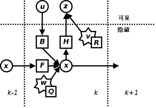

The filter can be confidently wrong
The equations are tidy; the engineering is less so. If wheel slip is much worse than the chosen Q, the filter may treat a mistaken motion prediction as reliable. If the camera occasionally locks onto the wrong landmark, a Gaussian measurement-noise model does not describe those outliers. Correlated sensor errors violate the independence assumption in the simple worked example. A badly calibrated R can give a poor sensor far too much authority.
The innovation offers a diagnostic. In the scalar example, its magnitude is 3 m and its predicted standard deviation is √(P + R) = √13 ≈ 3.61 m, so the normalized innovation is about 0.83 standard deviations. That observation is unsurprising under the model. A sequence of unexpectedly large innovations is evidence that the assumed uncertainties, dynamics or sensor associations deserve investigation. Rejecting every large innovation mechanically is also dangerous: a genuine abrupt manoeuvre could be mistaken for a faulty measurement.
For numerical robustness, implementations often use the Joseph covariance update, Pnew = (I − KH)Ppred(I − KH)ᵀ + KRKᵀ, instead of relying on the simpler algebraic form. Square-root filters propagate a factor of the covariance to better preserve its positive-semidefinite structure under finite precision. NASA’s 2008 comparison of nonlinear navigation filters discusses extended, square-root, UD and unscented approaches for lunar roving. The methods have different computational and accuracy trade-offs; none is universally best.
Nonlinear dynamics introduce another complication. An extended Kalman filter linearizes equations around the current estimate, which can fail when the approximation is poor. An unscented Kalman filter instead propagates selected sample points through the nonlinear model, at additional computational cost. Neither fixes a fundamentally wrong physical model or ambiguous data association.
A small reproducible test
Proposed simulation (not performed): Generate a one-dimensional trajectory with initial position 0 m, initial velocity 1 m/s, and 100 time steps of Δt = 0.1 s. Add independent Gaussian acceleration disturbances with standard deviation 0.2 m/s² at each step, using a specified random seed such as 42. Generate position observations every fifth step with Gaussian noise of standard deviation 1 m. Run a constant-velocity Kalman filter with state [x, v], initial covariance diag(4 m², 1 m²/s²), and a process-noise covariance derived from the chosen acceleration model. Plot true position, noisy observations, estimated position and the filter’s ±2σ position band.
Then deliberately underestimate measurement variance by a factor of 100 and repeat. Expect the filter to chase noisy measurements more aggressively, with intervals that often understate its actual errors. The exact curves depend on the random draw; this is a test proposal rather than a claim of observed performance. Check the fraction of true positions inside the nominal uncertainty band over many independent runs, not just one attractive plot.
For a historical foundation, see R. E. Kalman’s 1960 paper on linear filtering and prediction. NASA’s 1983 terminal-area navigation study provides a concrete aerospace example of combining position, air-data and acceleration sensors while managing computational constraints. On Alkemata, the earlier article on Gray code in position encoders addresses a different source of measurement error: transitions that can be misread before estimation even begins.
A useful navigation design therefore starts by asking two separate questions: what can the vehicle’s physics predict, and how uncertain is each observation? The Kalman equations combine the answers. Their precision is earned only when the uncertainty model survives contact with the real sensors.
Author
What concrete example would confirm or challenge this article?
Choose a reaction, write a comment, or ask your AI assistant to send a proposal for review. Comments are reviewed before publication.