Measuring temperature from a resistor’s random voltage

A precision thermometer can work without a sensing junction, a liquid column or a calibrated change in resistance. Connect a resistor to a sufficiently quiet measurement system and listen to its random voltage. The voltage has no repeating pattern. Yet its average squared amplitude reveals the resistor’s thermodynamic temperature.

The awkward part is that the measurement electronics also produce random voltage. The ingenious solution is to listen through two independent amplifiers and compare what they hear. Noise common to both channels survives; much of the noise generated separately inside each amplifier fades with averaging.

Why a resistor makes voltage with no battery

At nonzero temperature, mobile charges fluctuate inside a conductor. The fluctuations have zero mean, but they continually generate small terminal voltages. The equilibrium result is called Johnson–Nyquist noise. For an approximately ideal resistor in the classical, low-frequency regime, its one-sided open-circuit voltage-noise spectral density is

S_V = 4 k_B T R (V²/Hz).

Here k_B = 1.380649 × 10⁻²³ J/K is the Boltzmann constant, T is absolute temperature in kelvin and R is resistance in ohms. Over an effective measurement bandwidth B in hertz, with flat response and negligible loading, the mean-square noise voltage is 4k_BTRB, giving

V_rms = √(4 k_B T R B).

This equation contains the thermometer. If the resistance, bandwidth and measured noise power are known, temperature follows. The noise is an equilibrium property, which makes the technique attractive as a primary route to thermodynamic temperature rather than a measurement relying solely on a material’s empirical calibration curve. The 2019 NIST review of Johnson-noise thermometry describes both the physical foundation and the substantial measurement engineering required.

How small is the signal?

Take a hypothetical 100 Ω resistor at 300 K and an ideal 100 kHz measurement bandwidth. The predicted root-mean-square open-circuit noise voltage is about 0.407 µV. In a 1 Hz bandwidth, it is only about 1.29 nV. These are theoretical values, not measurements from an Alkemata experiment.

Notice that doubling temperature doubles noise power, but increases rms voltage by only √2. A small temperature change therefore produces an even smaller change in the voltage amplitude. Increasing bandwidth gathers more noise power, although the amplifiers and cables must maintain a well-characterised response across the wider band.

The apparent simplicity of the formula hides the main obstacle: an amplifier has its own input noise, and the cable can pick up interference. Simply connecting a voltmeter does not distinguish the resistor’s thermal fluctuations from the instrument’s contribution.

Two ears for the same random signal

Imagine that the resistor’s instantaneous voltage is s(t). Two separate amplifier chains produce measurements x(t) = s(t) + n₁(t) and y(t) = s(t) + n₂(t). The terms n₁ and n₂ represent the noise added by each chain. For this simple argument, assume the three signals have zero mean and that the amplifier noises are mutually independent and independent of the resistor noise.

Multiply the two measurements and average:

⟨xy⟩ = ⟨s²⟩ + ⟨s n₁⟩ + ⟨s n₂⟩ + ⟨n₁ n₂⟩ ≈ ⟨s²⟩.

The cross terms tend toward zero as independent samples accumulate. The shared resistor fluctuation remains. In a practical instrument, engineers compute a frequency-resolved cross-spectrum, reject unsuitable frequency regions, and integrate or fit the part that carries the thermal-noise signal. Averaging reduces the statistical uncertainty; it cannot remove systematic errors that appear identically in both channels.

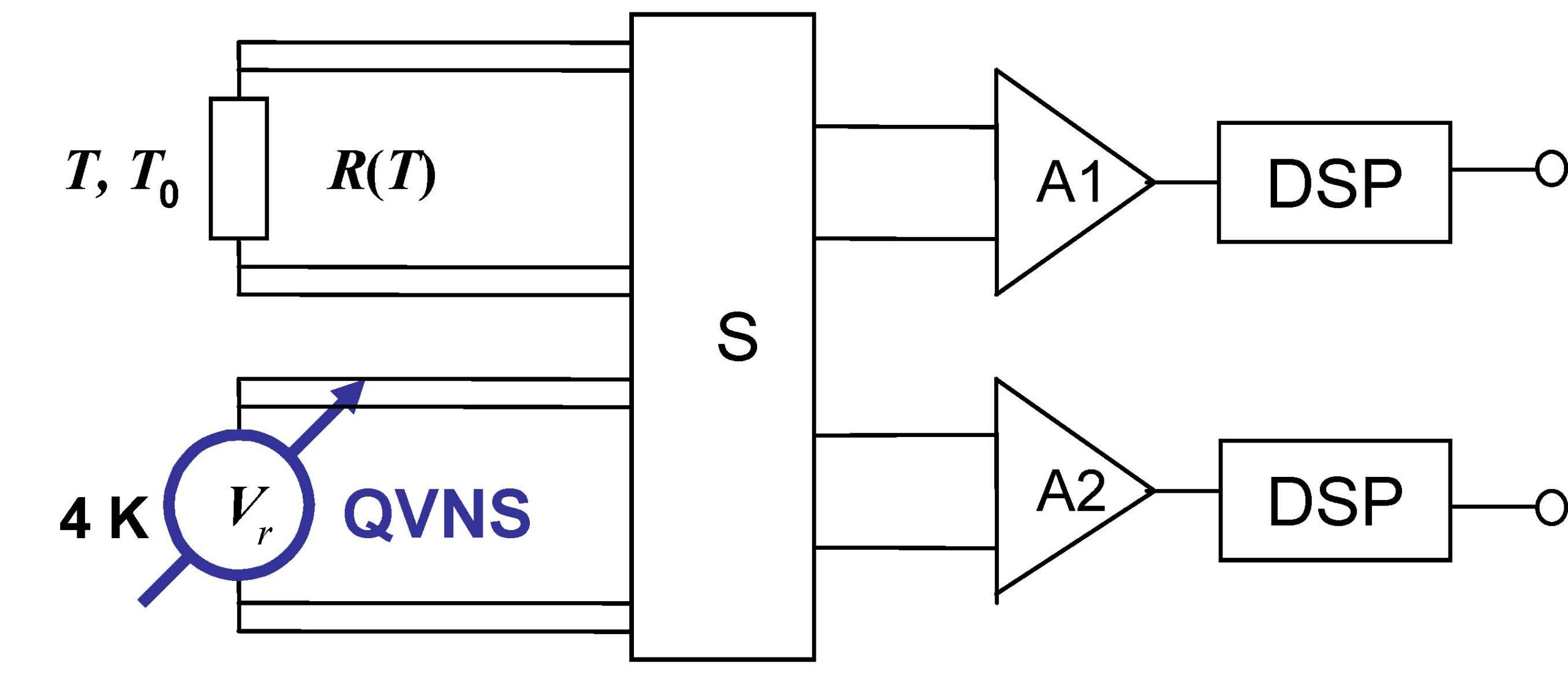
This is why two amplifiers can outperform one, even though the resistor signal itself is unchanged. The instrument deliberately duplicates the observation to identify what the two observations have in common.

The reference noise is engineered too

For primary metrology, measuring the resistor noise alone is insufficient: amplifier gain, frequency response and the precise effective bandwidth must also be known. NIST researchers address this by switching between the thermal resistor and a precisely synthesised quantum voltage-noise reference. The reference is built from Josephson-junction voltage technology and is designed to produce a calculable pseudo-random spectrum. Comparing the spectra largely cancels unknown common gain factors, provided the two signal paths are sufficiently matched.

The 2024 practical guide to realising the kelvin by Johnson-noise thermometry reports uncertainty around 1 mK near 300 K for the described primary method. It also makes the costs explicit: the quantum reference needs cryogenic operation, frequency responses of the resistor and reference leads must be matched, and measurement times are long. This is precision laboratory metrology, not a cheap replacement for a household thermometer.

One particularly revealing historical result comes from NIST’s 2017 determination of the Boltzmann constant. Researchers compared thermal noise against a quantum-accurate synthetic waveform, with a 100-day integration period, obtaining a relative standard uncertainty of 2.8 parts per million. The long averaging time illustrates how hard it is to extract a tiny statistical difference accurately.

Where correlation stops helping

The clean derivation assumed independent amplifier noise. Real channels can share power-supply interference, electromagnetic pickup, leakage through the source impedance or coupled input currents. Such correlated contamination remains in the cross-spectrum and can masquerade as resistor noise. Nonlinearities and frequency-dependent cable impedances also bias the inferred temperature. The NIST system description details how source design, filtering and spectral matching enter the uncertainty budget.

The classical expression also has a domain of validity. At sufficiently high frequency or low temperature, quantum corrections become important; a finite resistor and its leads may cease to behave like a frequency-independent lumped resistance. In ordinary audio and many radio-frequency bands at room temperature, the classical approximation is excellent, but an instrument’s own transfer function still needs checking.

There is also a subtle statistical limit. Cross-correlation suppresses independent additive noise in the mean; it does not make each finite-time estimate noiseless. The variance of the estimate falls with the number of effectively independent averages, so improving precision by a factor of ten can demand roughly one hundred times as much independent data under otherwise comparable conditions.

A small simulation worth running

Proposed simulation, not an experiment already performed: generate three independent zero-mean Gaussian sequences in Python. Give the common sequence a variance corresponding to 4k_BTRB for a chosen ideal bandwidth; give each amplifier sequence a larger variance. Form x=s+n₁ and y=s+n₂. Compare the single-channel mean squares with the sample average of xy as the number of samples grows. Then add a small shared interference sequence to both channels and observe the resulting persistent bias.

For a clean discrete-time demonstration, define the common signal variance directly and treat each generated sample as independent; a physical simulation would also model sampling rate, antialias filters, source loading and spectral shape. Plot estimate against sample count on logarithmic axes. Repeating the trial with different random seeds will show the spread of finite averages.

The most useful extension is to make the amplifier noises slightly correlated. How little coupling is enough to spoil a temperature estimate that aims for a part-per-million accuracy? That question leads directly from the simple algebra to the cable routing, shielding and reference switching of a real precision instrument.

The same instinct appears in Alkemata’s discussion of lock-in amplification: change the way a weak signal is observed so that unwanted contributions can be separated. A lock-in uses a known modulation reference; a noise thermometer uses a common random signal seen by two channels. The reference information is different, and so is the engineering.