
A photodiode measures a faint beam of light, but its output also contains electronic noise, temperature drift and interference. Turning up the gain amplifies all of them. A lock-in amplifier takes a more ingenious approach: make the light blink at a known rhythm, then ask which part of the detector signal keeps time with it.
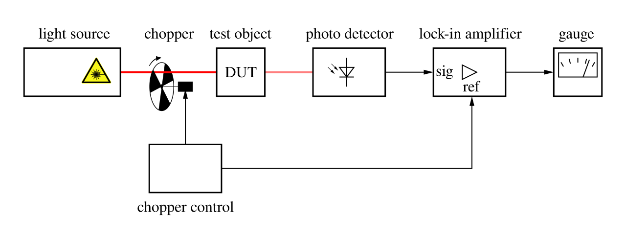
How to read the illustration: the chopper imposes a known rhythm on the light. A photodiode receives both the wanted modulated response and unwanted noise. The reference sent to the lock-in identifies the timing of the wanted response; inside the instrument, multiplication by that reference and low-pass filtering recover its amplitude and phase. The reference does not itself remove noise from the detector cable: it distinguishes components by their timing.
Move the information to a quieter frequency
Slow measurements compete with slow errors. Electronic offsets drift with temperature, and many devices exhibit 1/f noise that becomes stronger towards low frequencies. Instead of measuring a tiny steady photocurrent directly, interrupt the beam with an optical chopper or modulate an LED. The desired response now oscillates at a chosen frequency, perhaps 137 Hz. Slow drift remains near zero frequency. The exact frequency must be chosen to avoid local interference, mechanical resonances and the detector’s bandwidth limits.
The multiplication trick
Let the desired detector voltage be A cos(ωt + φ), where A is the peak amplitude, ω the angular frequency and φ the phase delay. Multiply the whole detector signal by a clean reference 2 cos(ωt). The wanted part becomes:
2A cos(ωt + φ) cos(ωt) = A cos(φ) + A cos(2ωt + φ)
A low-pass filter removes the rapidly oscillating term and retains the constant A cos(φ). Interference at a different frequency is shifted to the sum and difference frequencies; when the difference lies outside the filter bandwidth, the interference is rejected. This is synchronous demodulation. It measures correlation with a reference rather than the overall size of the noisy waveform.
Two reference waves remove a blind spot
A single channel fails if the response lags the reference by 90 degrees: cos(φ) is zero even though a signal exists. The solution is to multiply by two reference waves, separated by a quarter cycle. With a suitable sign and normalisation convention, the filtered outputs become X = A cos(φ) and Y = A sin(φ). The amplitude is √(X² + Y²) and the phase is atan2(Y,X). These are the in-phase and quadrature channels. Some instruments report root-mean-square instead of peak amplitude, so calibration conventions matter.
Phase is often valuable in its own right. A vibrating resonator shifts phase across resonance; heat diffusion produces a delay between periodic heating and the resulting temperature response; electrical impedance has resistive and reactive components.
Why sensitivity costs time
The low-pass filter rejects broadband noise by narrowing the measurement bandwidth. For white noise, the remaining root-mean-square noise scales with the square root of bandwidth. As an illustration, 100 nV/√Hz of input noise corresponds to roughly 10 µV across 10 kHz, but about 0.1 µV across 1 Hz, before accounting for mixing conventions and additional noise sources. A coherent 1 µV response may become measurable.
The price is slower settling and poorer tracking of fast changes. For a first-order low-pass filter with time constant τ, the −3 dB cutoff is 1/(2πτ). Different filters have different equivalent noise bandwidths and settling times. The instrument cannot undo detector saturation, insufficient analogue bandwidth or noise already introduced before digitisation.
When interference follows the same clock
The most deceptive error is an artefact synchronised with the reference. A chopper motor can inject electrical pickup at the chopping frequency; an LED driver may couple into the detector cable. The lock-in reports these artefacts faithfully because they keep time with the reference.
Good experiments therefore block the light while leaving the modulation electronics running, vary the reference frequency, test grounding, measure phase and compare a known reference sample. Near the noise floor, the non-negative magnitude √(X² + Y²) also has a positive statistical bias. Signed X and Y values and repeated background measurements give a more honest estimate of uncertainty.
The idea beyond one instrument
Lock-in detection is useful in spectroscopy, impedance analysis, scanning-probe microscopy and precision mechanics. It is a powerful example of experiment design doing part of the work that a more sensitive detector might otherwise have to do. It also illustrates a general caution: a clean instrument readout is not necessarily a validated measurement.
The deepest insight is a change of question: not “How large is everything the detector sees?” but “How much of it follows a pattern I deliberately imposed?” The next engineering challenge is proving that the pattern belongs to the phenomenon rather than the apparatus built to observe it.
Further reading and technical sources
- Stanford Research Systems, SR830 DSP Lock-In Amplifier manual — principles of phase-sensitive detection, quadrature channels, filters and time constants.
- Zurich Instruments, Principles of Lock-in Detection — practical mathematical explanation of modulation and demodulation.
- Wikimedia Commons: lock-in amplifier experimental setup — illustration origin and public-domain declaration.

