
Inside a magnetic-resonance instrument, millions of atomic nuclei contribute to one delicate electrical signal. The nuclei are not all in exactly the same magnetic field. Some rotate a little faster, others a little slower, and the combined signal rapidly fades. Building a perfectly uniform magnet would help, but there is a more elegant solution: let the spins drift apart, turn them over with a radio-frequency pulse, and wait for them to meet again.
The returning signal is a spin echo. It is not a reversal of time and not a recovery of information that has irreversibly disappeared. It is an ingenious way to separate two different reasons why a collective signal becomes weak: predictable loss of synchrony and genuine relaxation. That distinction has become foundational to nuclear magnetic resonance (NMR) and magnetic-resonance imaging (MRI). The original experimental account is Erwin Hahn’s 1950 paper, Spin Echoes.
Why a strong collection of spins can appear silent
Many nuclei, including hydrogen nuclei in water, possess a magnetic moment. In a strong magnetic field, the direction of this moment precesses, rather like a spinning top wobbling around a vertical axis. Its angular frequency is approximately ω = γB, where B is the magnetic field and γ is a property of the nucleus called its gyromagnetic ratio.
A radio-frequency pulse can tip the net magnetisation away from the field direction. After a nominal 90-degree pulse, the magnetisation has a component in the plane perpendicular to the main field. As that transverse component rotates, it induces a voltage in a receiver coil. The measured voltage is the collective contribution of many spins.
Here is the problem: the spins do not precess at precisely identical rates. Even a small spatial variation in the magnetic field produces slightly different frequencies. At first their transverse components point in much the same direction and add constructively. Later they fan out around the plane. The vectors can nearly cancel, although each individual spin is still precessing. The detector sees a weak signal, but part of the lost coherence is merely hidden in the distribution of phases.
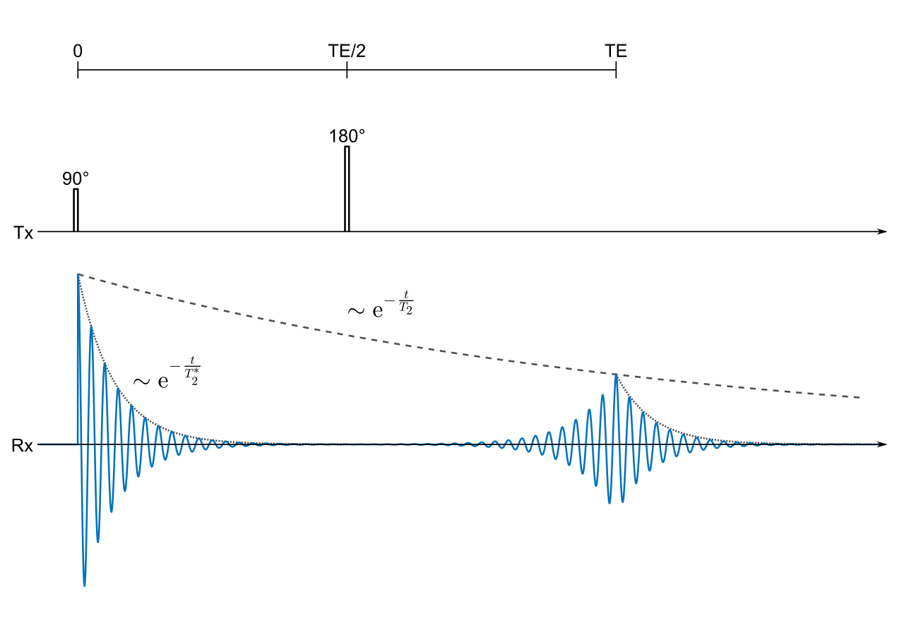
Magnetic-resonance practitioners distinguish the relatively fast apparent decay, often characterised by T2*, from the underlying transverse relaxation time T2. The former includes additional dephasing caused by static field variations; the latter reflects fluctuating microscopic interactions and other mechanisms that are not, in general, reversed by a single echo pulse. For an accessible technical discussion of this distinction, see the review of T2*-based magnetic-resonance imaging.
The clever intervention: flip the phases, not the frequencies
Imagine runners moving at different but constant speeds around a circular track. After a while they spread out. Simply telling everyone to stop would not restore their original positions. The useful trick is to exchange who is ahead and who is behind while leaving each runner’s speed unchanged. Given the same amount of time again, the faster runners catch up and the group reconvenes.
A spin-echo experiment implements a related geometric manoeuvre. First, a 90-degree radio-frequency pulse creates transverse magnetisation. The spins then freely precess for a delay τ. Next comes a 180-degree pulse, applied about a suitable axis in the rotating reference frame. This rotates each transverse spin vector so that its phase offset changes sign. The faster spins are now effectively behind the slower ones. Their frequencies have not changed, so during a second interval of length τ the phase differences shrink. At time 2τ after the first pulse, the transverse components come back into step and an echo appears.
The timing matters. The second pulse is not a new measurement and does not somehow force the nuclei to emit a delayed copy of the first signal. It changes the state of the ensemble so that the ordinary subsequent evolution causes constructive interference. A clinical MRI physics review illustrates how the 180-degree pulse reverses relative phase offsets while the underlying precession differences remain.
A two-line calculation explains the recovery
Consider a spin whose precession frequency differs from the reference by a constant amount Δω. During the first free-evolution interval it accumulates a relative phase φ = Δωτ. An ideal 180-degree pulse about the appropriate transverse axis maps that phase to -Δωτ. During the second interval, the unchanged frequency offset adds another +Δωτ. The result at the echo time is
φ(2τ) = -Δωτ + Δωτ = 0.
This cancellation works for every constant frequency offset, even when different spins have different offsets. For a numerical example, take one spin 10 Hz faster than the reference and another 10 Hz slower. After 25 milliseconds, their relative phases are respectively +90 and -90 degrees. The refocusing pulse exchanges those signs; after another 25 milliseconds both are back at zero relative phase. The echo peaks 50 milliseconds after excitation.
In the simplest ideal model, where the static offsets are fully refocused and transverse relaxation is exponential, the echo amplitude follows M(TE) = M(0) exp(-TE/T2), with TE = 2τ. Real samples and sequences can have more complicated decay. The crucial point is that the echo peak no longer contains the same uncontrolled attenuation from fixed frequency offsets that spoiled the initial free-induction signal.
What the echo cannot bring back
Calling this a reversal of time would be misleading. The 180-degree pulse changes spin orientations, not the sign of every interaction in the sample. If a spin’s local frequency changes between the two halves of the experiment, the two accumulated phases do not cancel exactly. Molecular diffusion through a magnetic-field gradient, motion, chemical exchange, fluctuating local fields and imperfect radio-frequency pulses can all reduce or distort the echo.
This limitation is useful rather than merely inconvenient. A measured echo is a selective test of what stayed predictable. It suppresses one class of experimental imperfection while leaving other physical processes visible. Carr and Purcell’s 1954 work examined diffusion and developed sequences with repeated refocusing pulses. Meiboom and Gill’s 1958 refinement addressed pulse-error accumulation by carefully choosing pulse phases. The family is commonly known as CPMG.
There is also a practical cost. A 180-degree pulse needs additional radio-frequency power, careful calibration and time. In clinical MRI, pulse sequences must balance contrast, acquisition speed, motion sensitivity and limits on deposited radio-frequency energy. A spin echo can be more robust against static field non-uniformity than a gradient echo, but it is not automatically the best choice for every imaging task. Conversely, sequences deliberately sensitive to field inhomogeneity or magnetic susceptibility can reveal information that a spin echo would partly suppress.
From correcting an error to measuring a material
The same idea serves two apparently opposite goals. In one experiment, an echo cancels unwanted static variations so that the remaining decay gives a more faithful estimate of transverse relaxation. In another, an experimenter deliberately applies controlled magnetic-field gradients. Molecules that diffuse between the gradient pulses fail to retrace the same phase history; their echo is attenuated. The loss becomes a way to infer molecular motion. A nuisance is turned into a measurement channel by choosing which part of the evolution to make reversible.
In MRI, pulse-sequence design similarly decides which physical differences between tissues should influence image contrast. The machine does not simply photograph the body. It engineers a succession of magnetic and radio-frequency interactions, then interprets the resulting signals. The spin echo is a particularly transparent example of this broader craft: good measurement often depends less on increasing detector sensitivity than on arranging the experiment so that the wanted information survives and the unwanted contribution cancels.
An experiment to try before touching an MRI scanner
The essential trick can be explored in a small simulation. Represent a thousand spins as arrows in a plane. Give each a different but fixed frequency offset, perhaps drawn from a bell-shaped distribution. Start every arrow aligned and plot the length of their vector sum as time passes: it collapses as the phases spread. At time τ, reflect each arrow’s angle across the reference axis to model an ideal 180-degree pulse. Keep the original frequencies. The vector sum returns to a peak near 2τ.
Now repeat with slowly changing frequency offsets, random phase kicks or a slightly imperfect flip. Which disturbances can be undone, and which cannot? That comparison is the deeper lesson. A clever physical intervention does not erase all errors; it makes some errors distinguishable from the phenomenon one wants to understand. The next question is whether other measurements could be designed around the same principle: instead of measuring a fragile signal more aggressively, can we arrange for the predictable disturbances to cancel themselves?
Sources and further exploration
The foundational papers are Hahn (1950), Spin Echoes, Carr and Purcell (1954), Effects of Diffusion on Free Precession, and Meiboom and Gill (1958), Modified Spin-Echo Method. For explanations of the imaging context, see Cardiovascular magnetic resonance physics for clinicians and Principles, Techniques, and Applications of T2*-based MR Imaging.

