
A controller can behave as if a forty-second delay were absent—without speeding up a sensor, a conveyor belt, or the laws of physics. It does so by controlling a carefully constructed prediction instead of blindly reacting to yesterday’s measurement. The trick is called the Smith predictor, and it is one of control engineering’s most elegant examples of solving a physical limitation with a mathematical rearrangement.
The surprising part is not simply “use a model.” Engineers do that everywhere. The ingenious step is to run two versions of the same model—one with the delay and one without—and subtract them in just the right place. That subtraction allows a conventional feedback controller to respond to a virtual, delay-free process while retaining a correction from the real plant.

Explore: when the machine answers too late
Imagine a factory rolling a strip of metal. The rollers adjust its thickness, but the gauge that measures thickness sits several metres downstream. If the strip travels at 0.5 metres per second and the gauge is 20 metres away, a change at the rollers cannot be observed by that gauge for 40 seconds. The delay is simply distance divided by speed: L = 20 m / (0.5 m/s) = 40 s.
A familiar proportional–integral (PI) controller compares the measured thickness with the target. If the measured strip is still too thick, its integral action keeps accumulating error and asking the rollers to close further. But for forty seconds, the gauge is reporting material that passed through before the latest adjustment. The controller may command another correction, then another, before the first one has even arrived at the sensor. Eventually the strip becomes too thin, the controller reverses, and an oscillation can follow.
This is dead time: a pure delay between a change in an input and its appearance in the measured output. It is different from a slow response. A slow heater may begin warming immediately but take minutes to reach a new temperature; a transport delay produces no visible response at the sensor until the material or information arrives. Many systems have both effects.
The traditional defence is patience: reduce controller gain, slow the integral action, and accept a less responsive process. But can we make the controller patient about the measurement without making it sluggish about the physics?
Understand: build two shadows of the process
O. J. M. Smith’s 1957 idea was to separate the plant into two conceptual pieces: its ordinary dynamics and a pure delay. A simple mathematical model is
P(s) = G(s) exp(-Ls),
where G(s) represents the delay-free dynamics, L is the dead time, and exp(-Ls) is the Laplace-domain representation of delaying a signal by L seconds. The variable s is the complex frequency used in linear-system analysis.
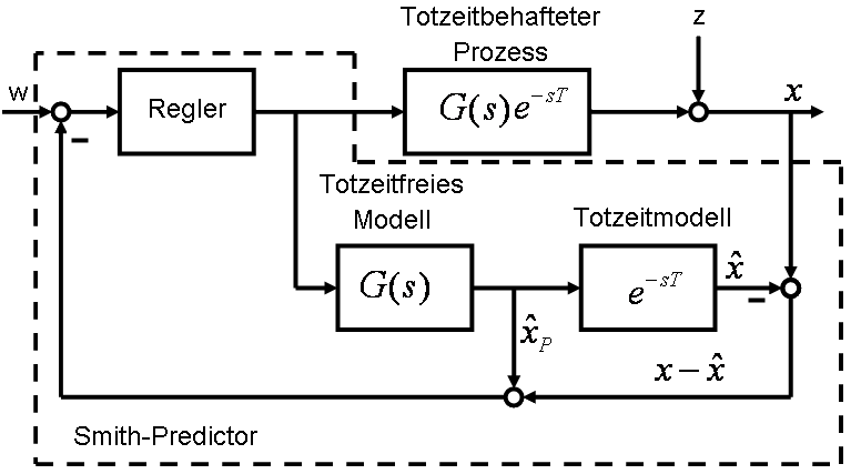
The predictor runs the controller’s command u through two internal paths:
- Fast shadow: the model
Ĝ(s)without its dead time producesŷ₀, an estimate of how the process would respond if transport were instantaneous. - Delayed shadow: the same model followed by the estimated delay
exp(-L̂s)producesŷL, an estimate of what the actual sensor should be reading now.
Then the real sensor value y is compared with the delayed shadow. Their difference y − ŷL is a model residual: whatever the delayed model failed to explain. Add that residual to the fast shadow and obtain the feedback quantity:
yfeedback = ŷ₀ + (y − ŷL).
That single line is the whole clever trick. The controller does not receive the stale measured value alone. It receives the model’s immediate estimate, corrected by the difference between reality and the delayed prediction. The measured signal is not discarded; it is used to challenge the model.
It is important not to call ŷ₀ a literal forecast of the actual sensor reading forty seconds in the future. It is the response of an imagined delay-free plant under the applied control history. In the ideal linear model, this is exactly the quantity that lets the controller be designed without putting transport delay inside its main feedback calculation.
Why the subtraction works
Suppose the model is perfect and no unmodelled disturbance is present. The actual sensor output equals the delayed prediction: y = ŷL. Therefore the residual is zero, and the controller sees simply yfeedback = ŷ₀. It can now be tuned against G(s), the delay-free part, rather than against G(s)exp(-Ls).
For a linear controller C(s) and setpoint r, the command obeys u = C(r − Gu) in this ideal case. Rearranging gives u = [C/(1 + CG)]r. The real output remains
y = exp(-Ls) [CG/(1 + CG)] r.
Notice where the delay went: it sits outside the familiar closed-loop factor CG/(1+CG). The controller can shape that factor as if it had no dead time, but the actual output is still shifted by L. The Smith predictor does not make a physical effect arrive sooner. It prevents the controller from repeatedly overreacting while waiting for it.
That distinction matters. A diagram showing an output beginning before the transport delay would be a diagram of a mistaken model, not a successful controller.
A numerical experiment: the two shadows disagree on purpose
Consider a normalized first-order process with time constant 20 seconds and a 40-second transport delay:
G(s) = 1/(20s + 1), L = 40 s.
To see the geometry of the prediction, apply a fixed unit step in the command at time zero; this is an open-loop demonstration, not a simulated closed-loop performance claim. The delay-free model responds as ŷ₀(t) = 1 − exp(−t/20) for t ≥ 0. The actual delayed process responds as zero for t < 40 s, then as y(t) = 1 − exp[−(t−40)/20].
| Time after command | Fast shadow ŷ₀ | Delayed sensor y (perfect model) | Residual y − ŷL |
|---|---|---|---|
| 20 s | 0.632 | 0.000 | 0 |
| 40 s | 0.865 | 0.000 | 0 |
| 60 s | 0.950 | 0.632 | 0 |
| 80 s | 0.982 | 0.865 | 0 |
The fast shadow has already risen substantially while the sensor still shows zero. That is not an error to be corrected by adding more actuator effort: it is exactly what the known transport delay predicts. Because the delayed shadow matches the sensor, their difference remains zero. The controller can “see” the effect of its own command in the model without being fooled by the old measurement.
In a real feedback loop, the command would change over time, and both models must be driven by the same actual command history. The table isolates the mechanism; it is not a promise that a particular PI tuning will settle in a particular number of seconds.
What happens when the real world refuses to match?
Suppose the gauge reports a thickness error that the delayed model did not predict. The residual y − ŷL is then nonzero and enters the feedback signal. This gives the controller a way to respond to disturbances, drift, and modelling errors rather than running indefinitely on an unchecked simulation.
But residuals cannot repeal causality. A disturbance that occurs at the rollers may itself take forty seconds to reach the gauge; the controller cannot infer an unknown disturbance before any evidence of it appears. Nor can the actuator undo a defect already moving downstream. Some implementations filter the residual to reduce noise and avoid overly aggressive corrections. That improves robustness but introduces its own speed–noise trade-off.
Where the trick earns its keep
The rolling mill is an unusually clear example because the transport delay can be estimated from distance and speed. The same logic applies to temperature control where heat or fluid must travel to a sensor, chemical processes with long residence or measurement times, and systems where communication or sensing adds substantial latency. A documented discrete-time Smith predictor implementation also illustrates motor-speed control with delayed feedback.
In practice, a Smith predictor is most attractive when the process is reasonably well described by a stable model and its delay is significant compared with its response time. If a better sensor location or a faster communication path can remove the delay, that physical change may be preferable. A clever controller should not become an excuse to ignore a simple engineering fix.
A concrete industrial test helps separate the concept from marketing. In a 2024 open-access study of a Brazilian iron-ore feeder–conveyor system, Moraes, da Silva and Euzébio compared a Smith predictor with the plant’s previous PID controller. Over the evaluated operating month, they reported a reduction of about 55% in the standard deviation of the flow-control error and an increase of about 355 tonnes per hour in tracked material flow. Those are site-specific observations, not a universal performance guarantee; the authors also found the predictor less robust to dead-time uncertainty in their simulations.
The trap: predicting the wrong delay
Imagine that the strip speed falls from 0.5 to 0.4 metres per second while the sensor stays 20 metres downstream. The real transport delay changes from 40 to 50 seconds. If the predictor still assumes forty, its delayed shadow begins responding ten seconds too early. The residual now contains a systematic discrepancy generated by the controller’s own inaccurate model. A feedback design tuned aggressively for the nominal delay can lose performance or stability.
Other errors matter too: changes in process gain, temperature-dependent dynamics, actuator saturation, sensor noise, nonlinearities, and disturbances entering at unexpected locations. For unstable or integrating plants, a textbook Smith predictor is not automatically appropriate; modified structures and robustness analysis are needed.
This is why industrial implementations often identify the process experimentally, retune when operating conditions change, filter residuals, constrain actuator commands, and test the controller against a family of plausible models. Research by Ingimundarson and Hägglund explicitly treats tuning and robustness under delay uncertainty. An engineering example from MathWorks shows how changing the residual filter trades some nominal speed for greater tolerance to model mismatch.
The subtle failure mode is epistemic: a predictor can give an excellent-looking internal signal while the physical system drifts away. The remedy is not to trust the model more, but to monitor its disagreement with measurements and retain conservative fallback behaviour.
Shape: try to break a virtual controller
Here is a useful small experiment for a classroom, a digital-twin prototype, or a control engineer with a simulator. No industrial equipment is required.
- Simulate a first-order plant with a 20-second time constant and a 40-second delay. Use a discrete time step much smaller than both, such as 0.2 seconds, and a delay buffer to store past commands.
- Implement a modestly tuned PI controller using only the delayed measurement. Apply a setpoint step; record settling time, overshoot, actuator excursions, and integrated absolute error.
- Implement a Smith predictor with the two model paths and the residual equation above. Tune the controller against the delay-free model, then compare the actual output, not just the virtual feedback signal.
- Repeat with true delays of 35, 40, 45 and 50 seconds while keeping the model delay fixed at 40. Add measurement noise, a load disturbance, and actuator limits. Do not claim one method “wins” unless you compare controllers at similar stability margins.
A particularly revealing plot would show three traces at once: the fast prediction, the delayed sensor value, and their residual. Under a good model, the first two traces look different but the residual remains near zero. When the model is wrong, the residual exposes the difference—possibly too late for an aggressive controller to recover.
That suggests a more ambitious design question: could a controller continuously estimate transport delay from operating speed, while refusing to act aggressively when its model becomes uncertain? Such a system would not merely predict; it would know when to distrust its prediction. That is a useful principle far beyond process control, from robotics to remote instruments and autonomous systems.
The idea worth keeping
The Smith predictor’s insight is not “ignore delay.” It is separate the predictable consequences of your own actions from the unexpected information in a measurement. A model supplies the first; the difference between observation and delayed model supplies the second. Used together, they can make feedback both more responsive and more intelligible.
But the physical delay is still there, and the model is still fallible. The best controller is not the one that pretends those facts have vanished. It is the one that makes them explicit—and can remain safe when its predictions are wrong.
Sources and further exploration
- O. J. M. Smith, “Closer control of loops with dead time,” Chemical Engineering Progress 53, 217–219 (1957). Bibliographic record of the original paper.
- A. Ingimundarson and T. Hägglund, “Robust tuning procedures of dead-time compensating controllers,” Control Engineering Practice 9, 1195–1208 (2001). DOI and Lund University research record. Primary research on tuning and delay uncertainty.
- MathWorks, “Control of Processes with Long Dead Time: The Smith Predictor.” Reproducible engineering example, model mismatch and filtering.
- M. Veronesi, “Performance Improvement of Smith Predictor Through Automatic Computation of Dead Time,” Yokogawa Technical Report (2003). Industrial implementation and variable delay.
- T. A. Moraes, M. T. da Silva and T. A. M. Euzébio, “Delay Compensation in a Feeder–Conveyor System Using the Smith Predictor,” Sensors 24, 3870 (2024). Primary industrial case study, open access.
- Control Engineering, “The Smith Predictor: A Process Engineer’s Crystal Ball” (1996). Accessible explanation using a rolling mill.
Author
What concrete example would confirm or challenge this article?
Choose a reaction, write a comment, or ask your AI assistant to send a proposal for review. Comments are reviewed before publication.