The One-Bit Converter That Pushes Its Errors Out of the Way

A precision sensor might produce a voltage that changes by only a few microvolts. A designer wants to turn that voltage into a reliable number, but a conventional analogue-to-digital converter (ADC) faces a difficult choice: build an exceptionally precise set of analogue thresholds, or accept errors from rounding the voltage to the nearest digital level. A surprising alternative begins with the crudest possible decision: is a signal above or below a threshold?

A sigma-delta converter can use that one-bit decision repeatedly to produce a much more precise measurement. The trick is not that each decision becomes accurate. It is that feedback makes the average decision track the input, while arranging for much of the rounding error to occur at frequencies the measurement does not need. A digital filter can then reject that unwanted part. This is noise shaping: not eliminating error, but moving it.

It is an instructive example of engineering by rearrangement. Rather than demanding perfect analogue components at every instant, the circuit trades speed, feedback and computation for precision over a limited bandwidth. The approach grew from telecommunications research, including Inose, Yasuda and Murakami’s 1962 delta-sigma modulation paper, and now appears in audio and precision measurement systems.

Explore: a coarse decision can still carry a fine measurement

Imagine measuring the average water level in a tank with a float switch that only reports “high” or “low”. One reading gives almost no precision. But suppose a controller continuously compares the actual level with the level implied by its previous decisions. When the estimate is too low, it tends to report “high”; when it is too high, it tends to report “low”. Over time, the proportion of high decisions can represent a level between the switch’s two states.

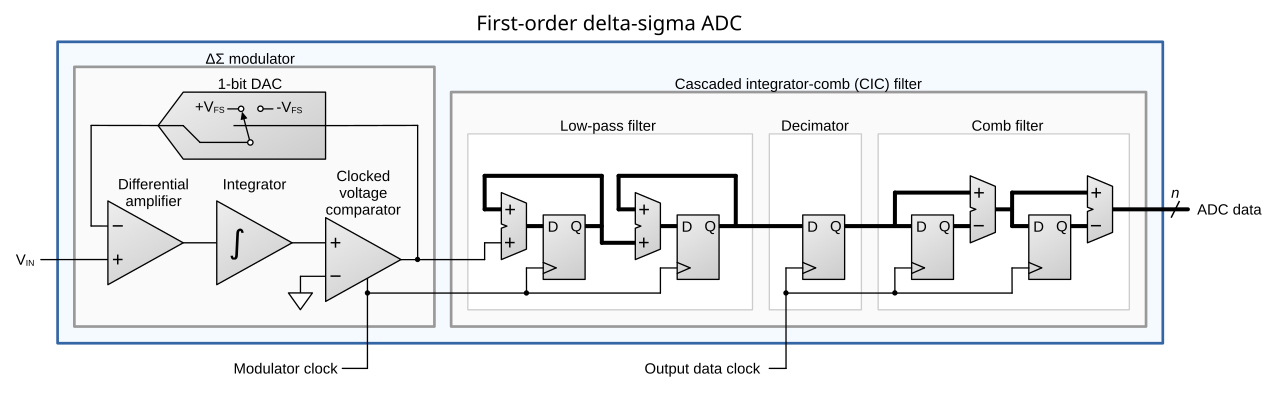
In a basic sigma-delta modulator, the switch is a comparator, the memory of accumulated mismatch is an integrator, and the controller closes a negative-feedback loop through a simple digital-to-analogue converter (DAC). The DAC converts the last output bit into one of two known analogue reference levels. That level is subtracted from the incoming signal. The integrator keeps a running account of the difference.

For an input normalised between −1 and +1, imagine the converter produces only +1 or −1 at each rapid clock tick. An input of +0.25 is represented, on average, by five +1 decisions and three −1 decisions in every eight decisions: (5 − 3)/8 = 0.25. The exact sequence and short-window counts depend on the loop state, but the long-term density of ones conveys a value far finer than one bit suggests. The individual bits are not binary digits of the final number.

The output looks noisy because it switches constantly. That appearance is not a defect to be removed at the analogue input. It is the deliberate raw material for a digital reconstruction step. Analog Devices’ comparison of ADC architectures describes this high-rate bitstream and the subsequent digital filtering and decimation.

Understand: the feedback loop remembers its mistakes

Consider a simple discrete-time model. Let x[n] be the input in units of the reference, y[n] the output decision (+1 or −1), and s[n] the integrator state. A convenient idealised update is s[n+1] = s[n] + x[n] − y[n]. The comparator chooses the next decision using the accumulated state, with timing chosen to keep the loop bounded. Real circuits implement the timing and analogue integration in different ways; this recurrence captures the central balance.

Now sum the update over N clock cycles. All intermediate integrator states cancel, leaving s[N] − s[0] = Σx[n] − Σy[n]. Rearranging gives average(y) = average(x) + (s[0] − s[N])/N. If the state stays bounded, the final correction shrinks as the observation window grows. This is the essential trick: the accumulated error cannot drift indefinitely without affecting the next decisions. The loop continually compensates for it.

That identity explains why a coarse output can preserve an accurate low-frequency average. It does not, by itself, guarantee an accurate waveform at every instant. For a changing input, the measurement needs a sufficiently fast modulator and a filter that retains the frequencies of interest. This is where sigma-delta goes beyond simply counting ones.

Simplified first-order delta-sigma ADC block diagram showing an integrator, one-bit comparator and feedback loop leading to digital output — A first-order sigma-delta converter: the integrator accumulates the mismatch between the input and a one-bit reference; the resulting bitstream is digitally filtered. Diagram by Lambtron, Wikimedia Commons, CC BY-SA 4.0, unmodified.

Where does the quantisation error go?

Ordinary quantisation rounds an analogue value to one of a finite set of levels. The difference is quantisation error. In the usual simplified analysis, a first-order sigma-delta loop is modelled as a linear system plus an additive error e[n] at the quantiser. Its output can be written approximately as Y(z) = X(z) + (1 − z⁻¹)E(z), allowing for an implementation-dependent sample delay in the signal path.

The two terms reveal different behaviour. The input passes through at low frequencies. The error is multiplied by 1 − z⁻¹, which corresponds in time to the difference between successive errors: e[n] − e[n−1]. Slowly varying errors almost cancel. Rapidly changing errors do not. On the unit circle, the magnitude is |1 − e^−jω| = 2|sin(ω/2)|. Near zero frequency it approaches zero; towards high frequency it becomes much larger. The loop has given the quantisation error a high-pass-shaped spectrum.

That is why the word shaping matters. The circuit does not abolish the rounding error or violate an information limit. It changes where in frequency the error is concentrated. The sensor’s slowly changing signal occupies a low-frequency band, while much of the error is pushed above it. A digital low-pass filter suppresses the high-frequency component; a decimator then produces fewer, more precise output samples. Analog Devices’ detailed topology explanation derives the signal and noise transfer functions, and Texas Instruments explains the practical digital filters.

Oversampling alone helps because a fixed amount of approximately white quantisation noise is spread over a wider frequency interval. In the ideal model, doubling the oversampling ratio improves in-band noise power by roughly 3 dB without shaping. For a first-order noise shaper, the idealised in-band quantisation-noise power falls approximately as the cube of the oversampling ratio, corresponding to about 9 dB improvement per doubling. Those are theoretical trends, not promised converter specifications: they assume a suitable quantisation-noise model and ignore other noise sources.

Why not use this trick for every signal?

The bargain works best when the signal occupies a relatively narrow bandwidth compared with the modulator clock. A slowly varying load-cell voltage, a temperature sensor or an audio signal may allow thousands of internal decisions for each useful output interval. A system that must capture an extremely fast transient, rapidly switch between many sensor channels or respond with very low latency may favour a successive-approximation (SAR) or another ADC architecture instead.

Filtering is not free. A sharper digital filter takes time to settle, so the converter may report a beautifully quiet value that describes the recent past rather than the present instant. If the input changes abruptly, the filtered output can lag. A digital filter also does not automatically prevent all analogue aliasing; unwanted signals near certain multiples of the modulator frequency can fold into the passband. Texas Instruments’ precision-ADC training discusses external noise, anti-alias filtering, clock jitter and reference-drive limitations.

Real modulators also have non-ideal integrators, finite reference accuracy, thermal noise, clock imperfections and limits on their stable input range. Simple one-bit loops can generate deterministic patterns, sometimes heard or measured as idle tones, rather than the perfectly random quantisation noise assumed in textbook formulas. Higher-order modulators shape noise more aggressively but make stability and overload behaviour harder to control. A high effective resolution in a narrow band is therefore not the same as an arbitrarily accurate instrument.

This distinction matters in applications. A digital weighing scale can display many digits, but the useful number of digits is limited by the load cell, temperature drift, vibration, reference stability, calibration and settling time—not merely the nominal bit count printed on the converter. The clever circuit creates an opportunity for precision; the measurement system must still earn it.

Shape: build a converter out of a running tally

The mechanism can be tested without analogue electronics. In a spreadsheet or short program, choose a constant input such as x = 0.25. Start with an integrator state of zero. At each tick, choose +1 when the current accumulated state plus the input is non-negative, otherwise −1; then update the state by adding x − y. Plot the resulting ±1 sequence, the running average and the integrator state. The bits look crude, but the running average converges towards 0.25 while the integrator stays bounded.

Next replace the constant with a slowly varying sine wave. Smooth the bitstream with a moving average and compare it with the original signal. Repeat with a shorter averaging window, then with a faster sine wave. You will see the fundamental trade-off: longer averaging suppresses more switching noise but blurs changes. A more realistic exercise uses a designed low-pass filter and inspects the power spectrum, distinguishing high-frequency quantisation error from low-frequency signal content.

For a fair comparison, repeat the exercise with a direct one-bit quantiser without feedback. Its output cannot track small analogue differences in the same way. Then deliberately overload the feedback loop or inject an out-of-band sinusoid. Which failure appears first: loss of tracking, delayed response, or contamination of the reconstructed signal?

The larger design question extends beyond converters. When an individual operation cannot be made precise, can a feedback system make the aggregate behaviour precise—and can the remaining errors be placed where they do the least harm? That question connects digital measurement to control, coding and many other forms of engineering. A related Alkemata article explores a different way of making weak signals measurable: the lock-in amplifier’s deliberate modulation.