Coriolis flowmeters: turning a tube’s twist into mass flow

A flowmeter sits in a pipe carrying a thick liquid. Its job is to report kilograms per second, even when the liquid warms, cools or changes composition. A conventional turbine or differential-pressure meter usually starts by estimating how much volume passes. To obtain mass flow, it also needs density. A Coriolis meter takes a different route: it makes a short section of pipe vibrate and watches how the moving fluid changes that vibration.

The measurable clue is surprisingly small. Two sensors on the tube report almost identical oscillations, but one arrives a little earlier than the other. The difference is calibrated into mass flow. The same vibrating tube can also provide a separate density estimate from its resonance frequency.

Why flow makes the tube twist

Picture a U-shaped metal tube fixed at its two ends. An electromagnetic drive excites a bending vibration, commonly near a mechanical resonance. In practical designs the drive and sensors are arranged to monitor a well-defined vibration mode; many meters use two tubes vibrating in opposite directions to reduce coupling to the surrounding pipework.

With no fluid moving through the tube, the inlet and outlet sections follow a symmetric oscillation. Fluid flowing through the U must continually change its direction and its motion relative to the vibrating structure. The inlet and outlet legs respond differently to that exchange of momentum: one tends to lag the driven motion, while the other tends to lead. The tube acquires a small twisting component superposed on its main oscillation.

The manufacturer Endress+Hauser’s explanation of the Coriolis measuring principle describes how pickup sensors at the two sides convert this twist into a time or phase difference. It is an instrumented elastic structure, not a miniature paddle wheel inside the fluid.

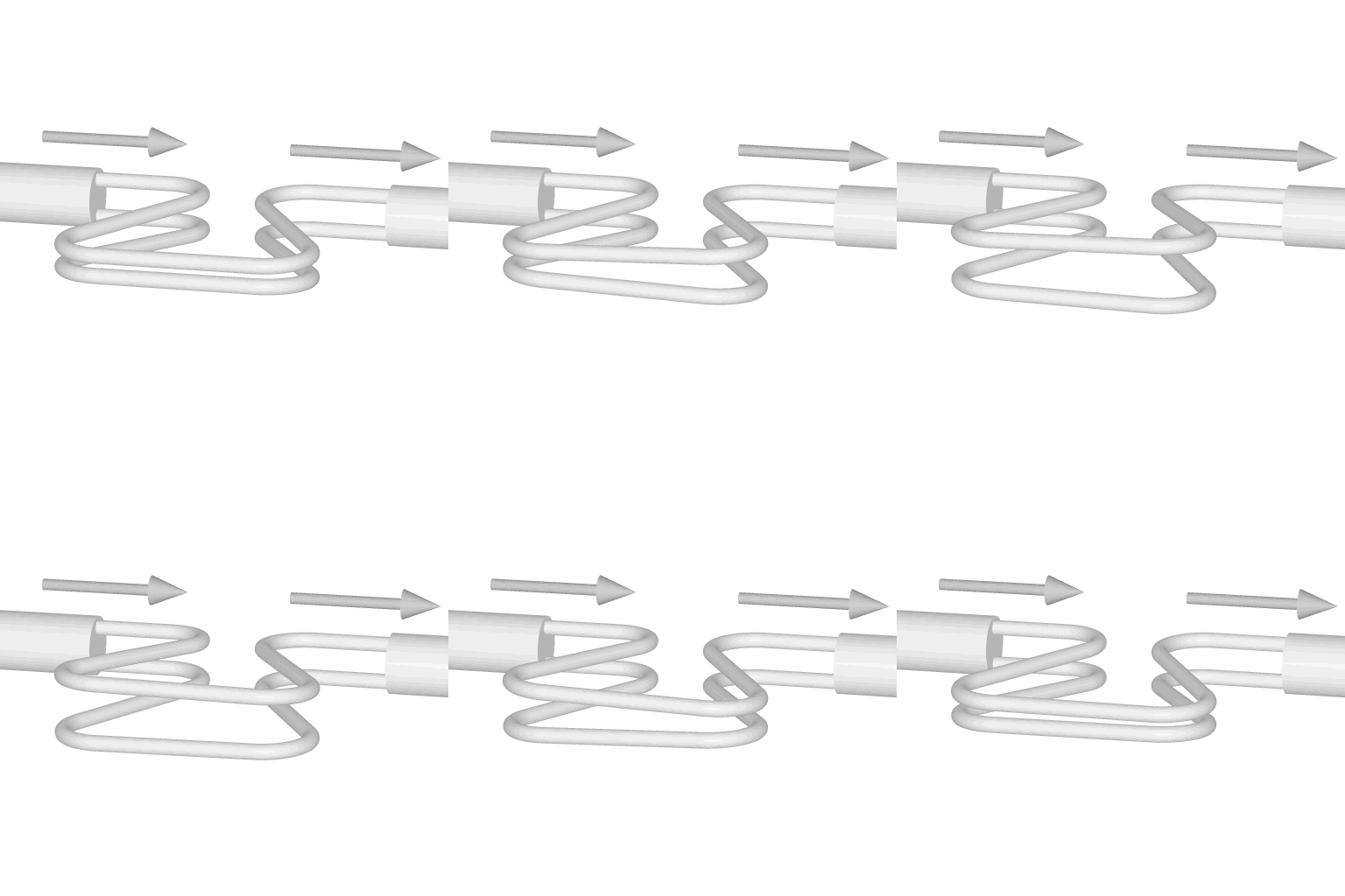
The momentum argument behind the measurement

Why should the deformation tell us about mass rather than just fluid speed? Take a small part of the tube that is instantaneously turning with angular velocity Ω. Fluid moving through that part with velocity v experiences a transverse acceleration in the tube’s moving frame. In the local rotating-frame approximation, its magnitude is

a_C = 2 Ω v,

when the two vectors are perpendicular. More generally, the acceleration is a vector cross product, 2 Ω × v, with the sign depending on the chosen frame convention. The tube must supply the corresponding transverse force to change the fluid’s motion; the fluid exerts the opposite reaction on the tube.

Consider a segment of length L, cross-sectional flow area A and density ρ. The fluid mass in that segment is approximately ρAL. Its Coriolis-force scale is therefore

F_C ≈ 2 ρAL Ωv = 2 ṁ L Ω,

where ṁ = ρAv is mass flow rate in kilograms per second. The units check: (kg/s) × m × (1/s) gives newtons. The key simplification is that density and velocity appear together as their product, mass flow. The force reverses direction with flow and with the oscillation.

This is a scaling argument, not a universal calibration equation. A real meter has a distributed elastic tube, curved geometry, moving fluid, damping, mode shapes and electronics. Its measured phase difference depends on all of these. A calibration maps the particular instrument’s time shift to kilograms per second, and the electronics compensate for changes in the tube’s mechanical properties.

How microseconds become kilograms per second

Suppose the inlet and outlet pickups produce near-sinusoidal signals at frequency f. The phase difference Δφ and time delay Δt are related by

Δφ = 2πf Δt (radians), or Δt = Δφ/(360° f) if the phase is expressed in degrees.

For an illustrative vibration at 100 Hz, a phase offset of 0.5° corresponds to Δt ≈ 13.9 microseconds. This number is a conversion between time and phase, not a claimed performance figure or a mass-flow calibration for a commercial meter. A zero-flow measurement establishes the baseline phase, and the instrument converts the flow-induced change into a signed mass-flow reading.

The technique is especially attractive when fluid density varies. For example, heating a liquid changes the volume passing through a given pipe section even if its mass delivery remains the same. A volume meter needs a reliable density correction to report kilograms per second. The Coriolis meter’s primary observable responds to the momentum transport associated with mass flow.

There is an important distinction here. The meter still needs calibration, and its indicated mass flow is not perfectly independent of temperature, pressure or fluid properties. Those influences can act through tube stiffness, damping and the measurement model, even though density is not required as a separate multiplier in the basic flow principle.

A second measurement hiding in the same vibration

Driving the tube near resonance gives another signal. A simple mass-and-spring oscillator has frequency f = (1/2π)√(k/m), where k is stiffness in newtons per metre and m is effective vibrating mass in kilograms. Fill the tube with denser liquid and the moving structure carries more inertia. Its resonant frequency generally falls.

Commercial Coriolis instruments use this relation, with a calibrated mechanical model, to estimate fluid density. Temperature sensors help correct changes in the tube’s elastic modulus. The electronics can therefore provide mass flow, density and temperature; volumetric flow can then be calculated as Q = ṁ/ρ when a meaningful bulk density is available.

The frequency trick has a close cousin in Alkemata’s article on the quartz crystal microbalance. Both exploit an inertial load changing a resonance, but the quartz device measures a thin attached film while the Coriolis instrument measures fluid flowing through a driven structure. For a different way of converting a tiny physical effect into phase, see the fiber-optic gyroscope.

What the clean principle leaves out

Two-phase mixtures are difficult. Bubbles or entrained gas change the apparent compressibility, damping and coupling of fluid to the tube, so a nominally direct mass-flow measurement can become biased. Abruptly varying flow can also challenge a sensor and its filtering. Coriolis meters are relatively expensive, introduce some pressure loss and require attention to vibration, installation stresses and zero stability, particularly near the bottom of their operating range.

Material stiffness matters more than the slogan “direct mass flow” might suggest. In a 2020 study, Fabio Costa, Jodie Pope and Keith Gillis at NIST tested a temperature-dependence model for a 5 cm dual-tube meter from 285 to 318 K. Their predicted temperature trend agreed with experimental results within 0.1% over that tested range. The authors examined how the elastic properties of the steel tubes affect the calibration, including the relevance of shear modulus. That result supports careful correction, not an assertion that every meter remains accurate at cryogenic temperature.

A separate NIST study of transient gas flow evaluated two commercial meters during a simulated gaseous-fuel filling operation. The investigators reported results against an independent transient-flow standard. It is a useful reminder that a meter’s behavior under changing conditions must be measured, not inferred solely from its steady-flow principle.

A testable timing exercise

Proposal, not a performed experiment. Generate two sampled sine waves at 100 Hz, with a sampling rate of 20 kHz. Give the second wave a phase offset of 0.5°, add independent zero-mean noise, and estimate the phase of each by fitting sine and cosine coefficients at the known drive frequency. Convert their difference to a time delay using the equation above. Repeat for 0°, +0.5° and −0.5°; then vary the record length and noise level.

The ideal expected delays are 0, +13.9 and −13.9 microseconds, subject to the chosen sign convention. Because a 20 kHz sample interval is 50 microseconds, estimating a delay smaller than one sample is possible only by using the waveform’s phase information across many samples. Longer records generally reduce random error for stationary uncorrelated noise, but they also average away fast changes. In a real flowmeter the mapping from this delay to mass flow still requires the tube’s mechanical response and calibration.

The engineering decision is now sharper: when a process demands mass rather than volume, a vibrating tube can avoid an external density correction. Whether that advantage outweighs pressure loss, cost, multiphase sensitivity and calibration demands depends on the fluid and the operating range.