The Magnetic Field That Keeps a Laser Braking Atoms

A beam of hot atoms can rush through a laboratory at hundreds of metres per second. How can one slow it to a walking pace using light? A laser can push against an atom, but the useful push seems to disappear as soon as the atom starts slowing. The reason is familiar: the Doppler effect. As the atom changes speed, the frequency of light it perceives changes too, and the atom falls out of resonance with the laser.

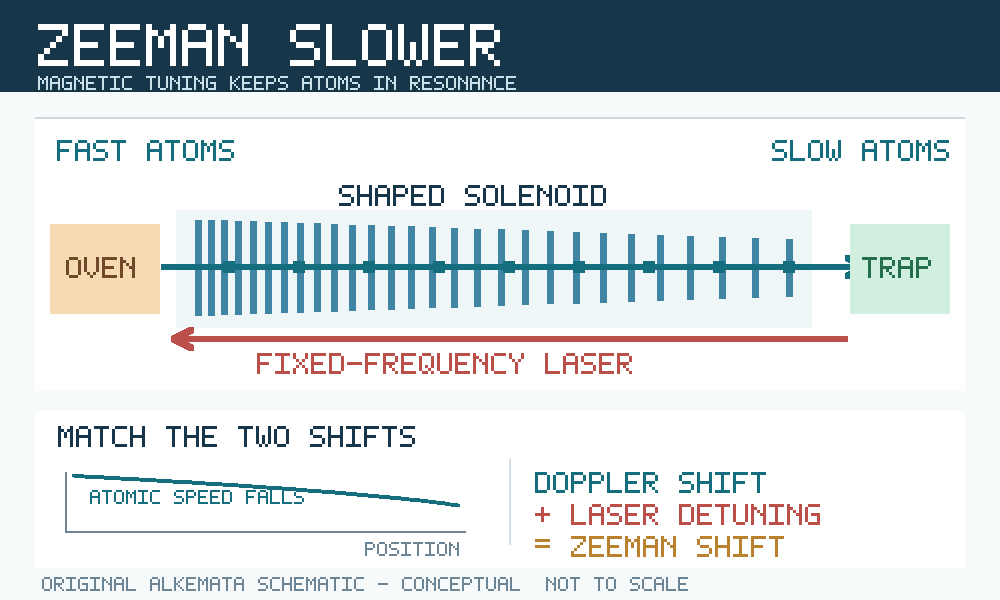
The surprising workaround is not to keep changing the laser. Instead, engineers change the atom’s resonant frequency as it moves. A carefully shaped magnetic field makes the atom stay tuned to one fixed-frequency laser all along its path. This device is called a Zeeman slower. It is an elegant case of using one physical effect to compensate for another.

Explore: light can brake matter, but only while it stays in tune

Consider a beam of neutral sodium atoms emerging from a hot oven into a vacuum system. They are not electrically charged, so ordinary electric fields cannot simply pull them to a stop. But each atom can absorb a photon from a laser tuned near one of its optical transitions. A photon carries momentum, even though it has no rest mass.

Arrange the laser to shine against the atomic beam. Every absorbed photon gives the atom a small backward momentum kick. The excited atom then emits a photon, generally in a random direction. Averaged over many cycles, the emitted photons contribute no preferred axial kick, while the absorbed photons keep pushing backwards. A single kick is tiny; thousands of repeated kicks are not.

Here comes the obstacle. Atoms absorb strongly only in a narrow frequency range. An atom moving toward the incoming laser sees the light Doppler-shifted upward in frequency. As the atom slows, that upward shift becomes smaller. A laser initially resonant with the fast atom soon becomes detuned. The atom stops scattering photons efficiently long before it stops moving.

One possible remedy is to continuously change the laser frequency as the atom slows, an approach called frequency-chirped slowing. But a continuous beam contains atoms at different positions and speeds at the same instant. A single laser frequency cannot be tailored independently to every atom. The Zeeman slower solves this spatially: it places different resonant conditions at different points along the beam.

Understand: the field shifts the atomic transition

The Zeeman effect is the shift or splitting of atomic energy levels in a magnetic field. For a suitably selected transition and a range in which its shift is approximately linear, we can write the transition’s angular-frequency shift as ω_Z(z) = μ_effB(z)/ℏ. Here B(z) is the magnetic field at position z, μ_eff is the effective difference in magnetic moments between the two levels, and ℏ is the reduced Planck constant.

Let the atoms move in the positive z direction, and let the laser propagate against them. Define the laser’s zero-field detuning as Δ = ω_L − ω₀, and let k = 2π/λ be the positive magnitude of its wave number. For a transition whose frequency increases with positive B, the atom’s approximate effective detuning is:

δ_eff(z) = Δ + kv(z) − μ_effB(z)/ℏ.

The kv term is the Doppler shift seen by the atom. The final term is the magnetic shift of the atomic resonance. The engineer chooses the coil profile so that these changing terms nearly cancel. Then δ_eff remains near the desired detuning, even as the atom loses speed.

This sign convention describes a decreasing-field slower with an appropriate choice of atomic transition. Other designs use an increasing field, a field that changes sign, or different magnetic sublevels. What matters is the matching, not that the field must always taper in the same direction.

For a constant target deceleration a, elementary kinematics gives:

v(z) = √(v_i² − 2az).

Substituting this into the resonance condition gives a practical design rule: choose B(z) so that μ_effB(z)/ℏ follows Δ + kv(z), allowing for an appropriate safety detuning. In the simple linear-Zeeman model, the field inherits a square-root profile. The coil is not merely a magnet; its winding distribution encodes a planned trajectory in velocity space.

The distinction is essential: the magnetic field is primarily the tuning mechanism. The average longitudinal braking force comes from the stream of absorbed laser photons. Confusing the two would give the wrong energy and momentum accounting.

How many photons does it take?

We can estimate the scale without building a complete quantum-optics simulation. Take a deliberately simplified sodium example: an initial speed of 600 m/s, a desired final speed of 100 m/s, and light near 589 nm. The momentum carried by one photon is p_γ = h/λ. The number of absorption events required to remove the desired axial momentum is approximately:

N ≈ m(v_i − v_f)λ/h ≈ 17,000 photons.

That sounds extravagant, but the recoil per photon is only about 0.03 m/s for sodium at this wavelength. Seventeen thousand small pushes add up to roughly 500 m/s of slowing. The result is an engineering estimate, not a promise that every atom in a thermal beam will complete the sequence.

Suppose we design for a constant mean deceleration of 3 × 10⁵ m/s². Then the required distance is:

L = (v_i² − v_f²)/(2a) ≈ 0.58 m.

The corresponding slowing time is (600 − 100)/a ≈ 1.7 milliseconds. A laboratory device less than a metre long can therefore make an enormous change in an atom’s speed. The calculation is idealised: it assumes that a suitable near-constant mean force is maintained throughout, and it omits recoil diffusion, collisions, transverse losses and details of sodium’s hyperfine structure.

What magnetic compensation is required? Over this 500 m/s speed change, the Doppler frequency changes by Δv/λ ≈ 849 MHz. A selected transition with a magnetic-frequency slope of about 1.4 MHz per gauss would therefore require a field change of roughly 600 gauss (0.06 tesla). The actual field profile depends on the transition, polarization, laser detuning and chosen operating margin. This illustrates why a spatially tailored solenoid is central to the device.

The deeper constraint: resonance does not guarantee enough force

Even perfect tuning cannot create unlimited braking. In the ideal two-level approximation, the average radiation-pressure force from a counterpropagating laser is

F ≈ −ℏk(Γ/2) × s/[1 + s + (2δ_eff/Γ)²],

where Γ is the spontaneous-decay rate in angular-frequency units and s is the laser saturation parameter. The negative sign denotes braking along the atom’s positive direction of travel. The force saturates as the excited-state population approaches its limit. More intensity eventually gives diminishing returns.

A useful design deliberately asks for less than the maximum possible deceleration. Why? If the designed field profile demands a speed reduction faster than the available optical force can deliver, an atom falls behind its intended trajectory in velocity space. Its detuning grows, scattering drops, and it can leave the slowing process altogether. A safety margin makes the trajectory more robust against changes in laser intensity, atomic velocity and magnetic field.

There is also a capture-velocity limit. Atoms that arrive too fast may never be close enough to resonance at the entrance. Others may be lost by imperfect polarization, optical pumping into unwanted states, beam divergence or collisions with residual gas. The output is not a perfectly monochromatic beam of atoms; it is a selected, slowed portion of an initial distribution.

Where this clever trick matters

A Zeeman slower is often placed between a hot atomic source and a magneto-optical trap (MOT). The slower provides atoms with sufficiently low forward velocity to be captured by the trap. The MOT then uses multiple laser beams and magnetic-field gradients to confine and cool atoms further. Slowing a directed beam and trapping a three-dimensional cloud are different jobs.

This distinction matters for experiments with ultracold gases, atomic clocks, precision spectroscopy and quantum simulation. Their performance depends not only on sophisticated downstream optics, but also on how many useful atoms the source delivers. A poorly designed slower can waste an excellent atomic source; a robust one can substantially improve loading without changing the trap itself.

The historical evidence is unusually clear. In March 1982, William D. Phillips and Harold Metcalf reported slowing a sodium beam by approximately 40% of its initial thermal velocity, corresponding to about 15,000 absorptions. Later that year, John V. Prodan, Phillips and Metcalf reported sodium atoms slowed to about 40 m/s. The first result established the compensation method; the later experiment showed how far the technique could be pushed. Both are measured results, distinct from the illustrative numerical design above.

Shape: a field profile is a control program written in space

The general engineering lesson reaches beyond atomic physics. A moving object changes the conditions under which it responds to a control input. Rather than continuously retune the input, we can arrange the environment so that the object encounters the right condition at the right place. The Zeeman slower turns a spatial magnetic-field profile into a passive schedule for an atom’s evolving speed.

It is a close conceptual cousin of other strategies that compensate for a changing operating condition rather than overpowering it. In Alkemata’s earlier exploration of chirped-pulse amplification, a laser pulse is deliberately stretched before amplification and compressed afterward. In both cases, a constraint becomes manageable by changing the path through which a process evolves.

A practical thought experiment: imagine designing two slowers for the same sodium beam. One uses a constant magnetic field; the other uses B(z) to track v(z). Plot the detuning δ_eff against distance for both. Then shorten the shaped slower by 30% while keeping its entry and exit speed targets. Does it still work? Only if the optical force can sustain the extra required deceleration. This separates the resonance constraint from the force constraint.

And it raises a broader design question: when a machine seems to need an ever-faster controller, could some of the required intelligence instead be built into its geometry, material, or field distribution?

Sources and further exploration

• W. D. Phillips and H. Metcalf, “Laser Deceleration of an Atomic Beam,” Physical Review Letters 48, 596–599 (1 March 1982). Original experimental demonstration.
• J. V. Prodan, W. D. Phillips and H. Metcalf, “Laser Production of a Very Slow Monoenergetic Atomic Beam,” Physical Review Letters 49, 1149–1153 (18 October 1982). Follow-up experimental result.
• W. D. Phillips, “Nobel Lecture: Laser cooling and trapping of neutral atoms,” Reviews of Modern Physics 70, 721–741 (1998). Historical and technical review.
• U.S. National Institute of Standards and Technology, “Context of a Discovery: Bill Phillips.” Institutional account of the tailored-solenoid solution and experimental history.
• L. Zhao, J. Jiang and Y. Liu, “Optimizing a spin-flip Zeeman slower” (2014). Later design and robustness considerations.