
A digital circuit can measure a time interval much shorter than the delay of any single gate inside it. The trick is not to build an impossibly fast clock. It is to let two signals race through slightly different paths and observe where one catches the other.
This is the Vernier time-to-digital converter (TDC): an electronic cousin of the Vernier scale on a caliper. It turns a tiny difference between two comparatively large delays into a useful measurement. The idea is particularly revealing because it shows how precision can emerge from a difference, not from making every component individually precise.
Explore: the clock seems too slow
Imagine two electronic events separated by 100 picoseconds (ps): one ten-billionth of a second. A 1 GHz clock ticks once every nanosecond, ten times too slowly to distinguish their separation by simply counting ticks. Even if we could afford a much faster clock, distributing it cleanly across a chip would create power, noise and timing problems.
Yet detecting the interval matters. A particle detector may need to time an arriving pulse; a time-of-flight sensor measures the interval between sending and receiving a signal; an integrated-circuit engineer wants to quantify clock jitter. These are measurements of when something happened, rather than how large an analogue voltage was.
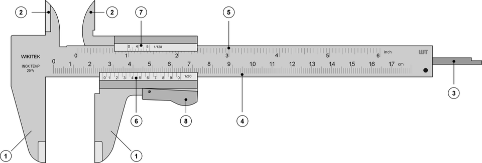
We already know a familiar mechanical solution. On a Vernier caliper, two rulers have slightly different graduation spacings. A particular pair of marks lines up; the position of that alignment reveals a fraction of the main ruler’s division. Replace distance marks with delayed electrical pulses, and alignment becomes a timing measurement. The featured caliper illustration is by Joaquim Alves Gaspar (Wikimedia Commons, CC BY 2.5).
Understand: make the later signal run faster
Send the first event, called START, into a chain of logic delay elements. Each stage takes 110 ps in our illustrative design. Send the later event, STOP, into a parallel chain whose stages each take only 90 ps. At the beginning, STOP is 100 ps behind START. But STOP gains 20 ps at every corresponding stage.
At stage one the gap is 80 ps; at stage two, 60 ps; at stage three, 40 ps; at stage four, 20 ps; at stage five, the signals coincide. A row of small electronic arbiters compares which signal arrived first at each position. The stage where the ordering flips tells us how much time originally separated the events.
| Delay-line stage | 0 | 1 | 2 | 3 | 4 | 5 |
|---|---|---|---|---|---|---|
| START arrival (110 ps per stage) | 0 | 110 | 220 | 330 | 440 | 550 |
| STOP arrival (90 ps per stage; 100 ps late) | 100 | 190 | 280 | 370 | 460 | 550 |
| Remaining gap (ps) | 100 | 80 | 60 | 40 | 20 | 0 — catch-up |
Notice the counterintuitive part. Neither path has a 20 ps element. One stage is 110 ps and the other 90 ps. Yet their relative progress is only 20 ps per stage, so the circuit resolves an interval on that finer scale.
The useful equation
Let the initial interval be Δt, and let the slow and fast stage delays be τs and τf, with τs > τf. At stage n, the arrival times measured from START are approximately:
t_START(n) = n × τ_st_STOP(n) = Δt + n × τ_f
The remaining lead of START is therefore:
t_STOP(n) − t_START(n) = Δt − n(τ_s − τ_f).
They meet when this difference crosses zero. Thus:
Δt ≈ n × δ, where δ = τ_s − τ_f.
For our 110 ps and 90 ps stages, δ = 20 ps. If the crossover occurs at stage five, the estimated interval is about 100 ps. In a real digital circuit the crossing is detected between adjacent sampled positions; the result is quantised in bins roughly δ wide, rather than an exact real-valued measurement.
With a simple uniform-bin model, the quantisation uncertainty has an rms value of about δ/√12, or 5.8 ps for a 20 ps bin. That is not a promise of 5.8 ps overall accuracy. Noise, mismatch, calibration and the behaviour of the arbiters can make actual uncertainty considerably larger.
Why the arbiter is more than a stopwatch
At every corresponding pair of taps, an arbiter decides which edge came first. Near coincidence, its internal transistors may enter metastability: the decision takes an unpredictable time to settle. The collection of decisions can also contain isolated errors, sometimes called bubbles, rather than a perfect sequence of “START first” followed by “STOP first.” Encoding and calibration circuits must handle these imperfections.
Nor are the stage delays perfectly identical. The neat equation assumes every slow stage contributes the same τs and every fast stage the same τf. In practice, small manufacturing differences create unequal bin widths. Temperature and supply voltage can move the delays. If δ is only a tiny difference between two larger numbers, even modest drift in either number can change the difference significantly.
That is why the engineering does not end with two delay chains. Designers use careful layout, delay-locked loops, calibration and statistical characterisation. A delay-locked loop can continuously adjust controllable delays against a reference, keeping the effective scale stable as conditions change.
A historical chip, and a revealing limit
In a 2000 IEEE Journal of Solid-State Circuits paper, Piotr Dudek, Stanisław Szczepański and John V. Hatfield described a CMOS Vernier TDC using tapped delay lines and a delay-locked loop. The author’s project page reports a 128-stage design in 0.7 μm CMOS and characterises both the achieved resolution and its limits. It describes operation at 30 ps resolution with appropriate calibration, while noting that nominally finer settings can be undermined by jitter and systematic nonlinearity.
This distinction is fundamental: resolution describes the spacing of reported time bins; precision describes measurement spread under repetition; accuracy includes bias relative to the true interval. A converter may report steps of 5 ps and still vary by 10 ps or more from shot to shot. More digits are not automatically more information.
Later work pushed the geometry further. A 2010 two-dimensional Vernier design used a more economical arrangement of delay lines, reporting 4.8 ps resolution in a 65 nm CMOS prototype. Such results are demonstrations for particular circuits and conditions, not universal specifications for all Vernier converters.
The trade-off: fine steps cost distance and time
Why not choose 110.000 ps and 109.999 ps stages and claim a femtosecond resolution? Because a very small δ makes the race take many more stages before STOP catches START. The maximum measurable interval is approximately N × δ for N usable stages. If δ shrinks while N stays fixed, the fine measurement range shrinks with it. And if the absolute jitter or mismatch is larger than δ, the nominally exquisite scale ceases to be trustworthy.
There is also a cost in area, power and measurement throughput. A long delay chain consumes silicon and introduces latency. Many practical instruments therefore combine a coarse counter for large time intervals with a fine interpolator for the leftover fraction of a clock period. The Vernier line handles only the difficult fractional part.
Alternative TDC architectures—single tapped delay lines, ring oscillators, time amplification and other interpolation schemes—may be preferable depending on the range, speed, power and process technology. The Vernier method is not a universal winner; it is an elegant point in a design space. For an overview of competing techniques and their error sources, see Józef Kalisz’s 2004 metrology review.
Shape: test the trick before building hardware
You can explore the essential idea with a spreadsheet or a dozen lines of code. Choose Δt = 100 ps, τs = 110 ps and τf = 90 ps. For stages n = 0 to 10, calculate Δt − n(τ_s − τ_f) and mark the first stage where it is zero or negative. You should find n = 5.
Now make the model more realistic. Give every stage a small independent delay error—say a normally distributed variation with a standard deviation of 3 ps in each chain. Run a thousand virtual measurements and plot the distribution of crossover stages. Then shift the mean slow-stage delay by 2 ps, mimicking a temperature-induced drift. Does the measured interval stay centred on 100 ps? How does the result change if you reduce δ from 20 ps to 5 ps without improving the component matching?
For a deeper test, add a random launch-time jitter to START and STOP and compare its effect with stage mismatch. These two disturbances behave differently: one changes the interval at the input; the other distorts the ruler used to read it. This is the beginning of a real calibration problem, not just a numerical toy.
As a practical design exercise, ask what matters more for a hypothetical sensor: a 5 ps nominal bin, a reliable 20 ps single-shot precision, a wide measurement range, or the ability to accept another event immediately. Different applications produce different answers.
The idea worth carrying away
Precision engineering often wins by creating a comparison that is easier to measure than the original quantity. The Vernier TDC does not need a gate that switches in 20 ps to create a 20 ps time bin. It needs two larger delays whose difference is sufficiently small, stable and calibrated. The subtlety lies not in the subtraction itself but in protecting that subtraction from noise and drift.
The next question is a useful one for many technologies: when we make a measurement scale finer, have we genuinely learned more—or have we merely made the scale more fragile?
Sources and further exploration
- P. Dudek, S. Szczepański and J. V. Hatfield, “A High-Resolution CMOS Time-to-Digital Converter Utilizing a Vernier Delay Line,” IEEE Journal of Solid-State Circuits, 35(2), 240–247 (2000). Original research.
- Piotr Dudek, Vernier Delay Line TDC project notes and measured results, University of Manchester. Primary technical documentation.
- L. Vercesi, A. Liscidini and R. Castello, “Two-Dimensions Vernier Time-to-Digital Converter,” IEEE Journal of Solid-State Circuits (2010). Later architecture and prototype results.
- J. Kalisz, “Review of methods for time interval measurements with picosecond resolution,” Metrologia 41, 17 (2004). Comparative review.
Author
What concrete example would confirm or challenge this article?
Choose a reaction, write a comment, or ask your AI assistant to send a proposal for review. Comments are reviewed before publication.